This is a blog post based on my presentation at the Amsterdam Python Meetup, June 2014 over at the guys from Byte

Background

• Human Movement Scientist
• Specialized in gait analysis and pressure measurements
• Pythonista, Matlab-survivor and reluctant R-user

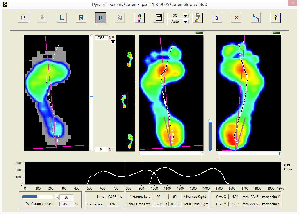
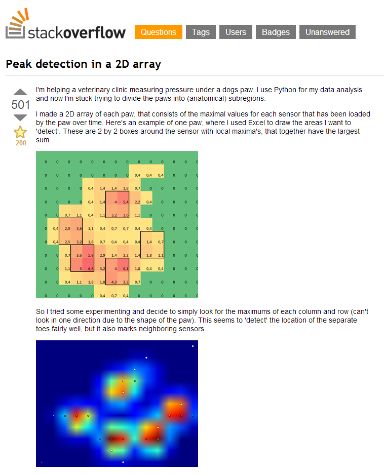
Normally pressure measurements are done on humans using a pressure plate. In this case we used a 200x36 cm pressure plate, it has 256x64 sensors which measure at 126 Hz. When you walk over it, each sensor measures the force applied to them and after interpolation, you get these nice looking pressure measurements.

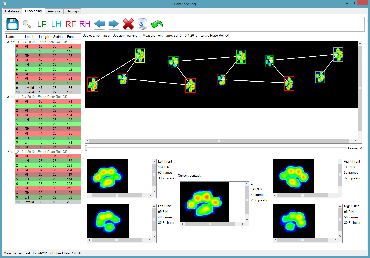
But I needed a version that worked on animals too. The regular software doesn't work on animals, due to several limitations (not detecting the paws being a major one).

So I created Pawlabeling, see Github: https://www.github.com/ivoflipse/pawlabeling

Its called Pawlabeling, because its used to label paws. Who ever said naming hard to be hard?!?

Scientific Python stack

The application uses a lot of libraries from the scientific python stack:

• PySide (GUI)
• NumPy (array operations)
• SciPy (scientific calculations)
• PyTables (storage)
• OpenCV (computer vision)
• Matplotlib (plotting)
• Scikit-Learn (machine-learning)

For installing I recommend Anaconda (Continuum Analytics) or Canopy (Enthought).

Interesting problems

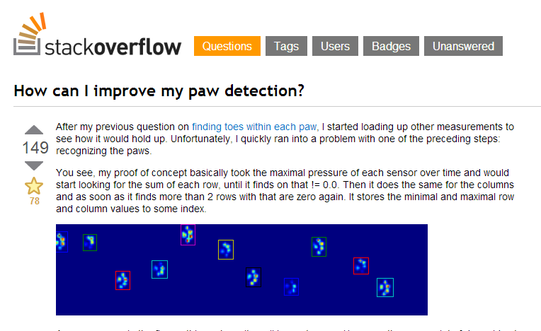
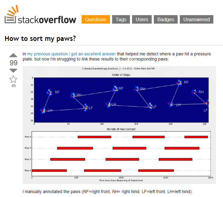
While working on this project I ran into lots of interesting problems and like any junior developer: you go to Stack Overflow! Luckily the Python community is awesome and especially Joe Kington's answers helped me a lot (all his Matplotlib answers too BTW).

• Detection and tracking of paws

• Labeling the paws

• Detecting toes

Focus of the talk

Today, I'll just be focusing on the problem I'm working on right now: Labelingthe paws.

Given the data of a paw, predict its label (LF, LH, RF, RH)

So how can we solve this?

Let's use Machine Learning

Gael Varoquax (scikit-learn developer):

Machine Learning is about building programs with tunable parameters that are adjusted automatically so as to improve their behavior by adapting to previously seen data.

Today we'll focus on Supervised Learning:

Supervised learning consists of learning the link between two datasets: the observed data X and an external variable y that we are trying to predict, usually called target or labels. Most often, y is a 1D array of length n_samples.

Like finding a line that separates these black and white points

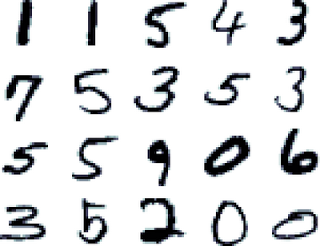
Or predicting the digit given an small image of a digit, like in the MNIST dataset:

If you have no clue what algorithm to use, you should read the documentation first or just use the Scikit-Learn cheat-sheet:

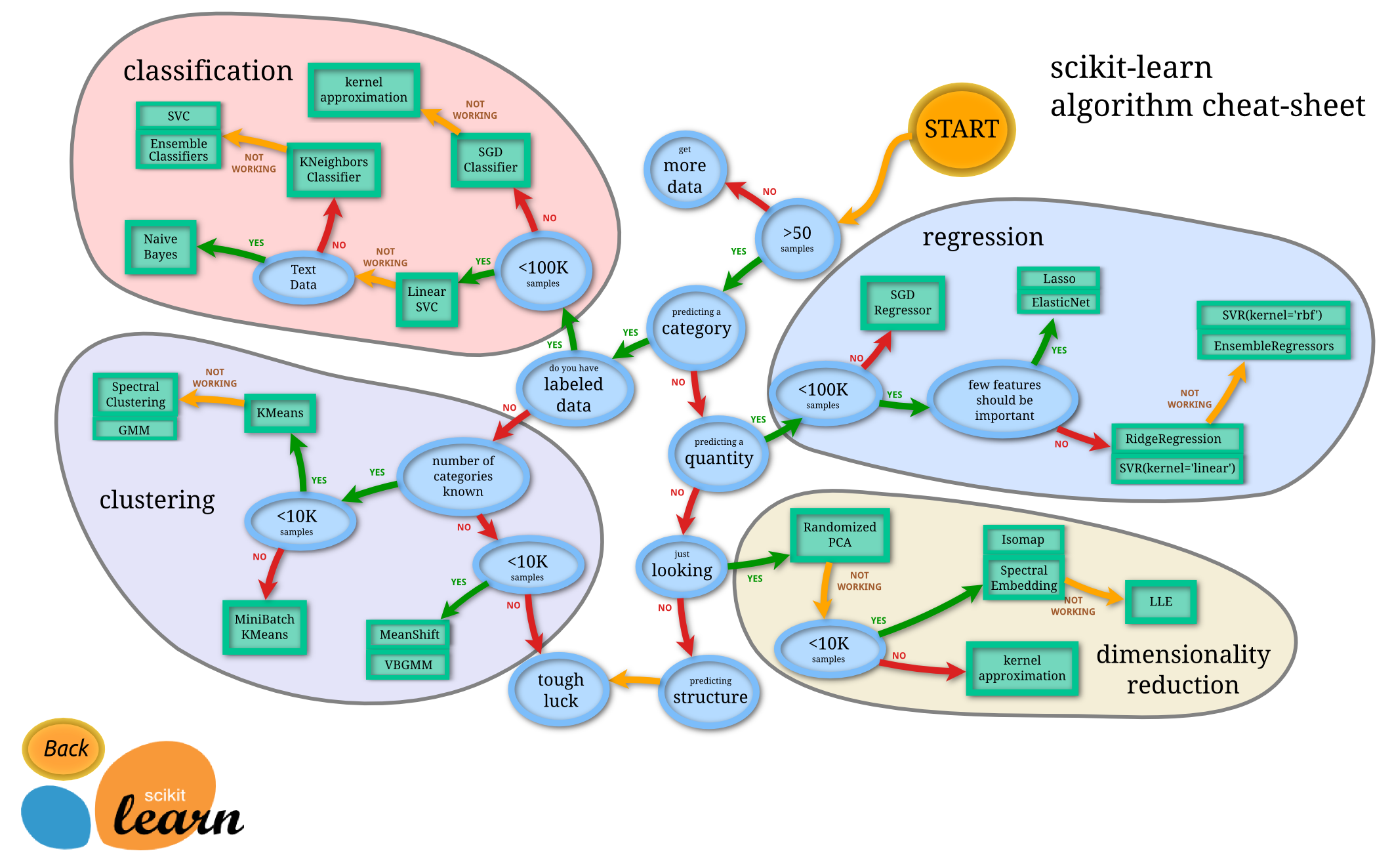
Source: Andreas Müller

Starting at Start:

• Yes, I have more than 50 samples
• Yes, I'm trying to predict a category
• Yes, I even have lots of labeled data (its called Pawlabeling for a reason d'uh!)
• Darn, I don't have more than 100k samples
• I could use a Linear Support Vector Classifier, but why stop here?
• No, I don't have text data
• Meeh, I don't want to use KNeighbors Classifiers
• So we end up at Ensemble Classifiers (ignoring the Support Vector Classifiers)

From the Ensemble Classifiers, I randomly picked the Random Forest classifier

Random Forests

Why use Random Forests:

• Easy to use
• Used for regression (predicting values)
• Used for classification (predicting categories)
• Gives you good scores on (entry-level) Kaggle competitions :-)

I thought I'd add this Quora question as a note, that explains Random Forests in laymans terms:

Suppose you're very indecisive, so whenever you want to watch a movie, you ask your friend Willow if she thinks you'll like it. In order to answer, Willow first needs to figure out what movies you like, so you give her a bunch of movies and tell her whether you liked each one or not (i.e., you give her a labeled training set). Then, when you ask her if she thinks you'll like movie X or not, she plays a 20 questions-like game with IMDB, asking questions like "Is X a romantic movie?", "Does Johnny Depp star in X?", and so on. She asks more informative questions first (i.e., she maximizes the information gain of each question), and gives you a yes/no answer at the end.

Thus, Willow is a decision tree for your movie preferences.

But Willow is only human, so she doesn't always generalize your preferences very well (i.e., she overfits). In order to get more accurate recommendations, you'd like to ask a bunch of your friends, and watch movie X if most of them say they think you'll like it. That is, instead of asking only Willow, you want to ask Woody, Apple, and Cartman as well, and they vote on whether you'll like amovie (i.e., you build an ensemble classifier, aka a forest in this case).

Now you don't want each of your friends to do the same thing and give you the same answer, so you first give each of them slightly different data. After all, you're not absolutely sure of your preferences yourself -- you told Willow you loved Titanic, but maybe you were just happy that day because it was your birthday, so maybe some of your friends shouldn't use the fact that you liked Titanic in making their recommendations. Or maybe you told her you loved Cinderella, but actually you really really loved it, so some of your friends should give Cinderella more weight. So instead of giving your friends the same data you gave Willow, you give them slightly perturbed versions. You don't change your love/hate decisions, you just say you love/hate some movies a little more or less (you give each of your friends a bootstrapped version of your original training data). For example, whereas you told Willow that you liked Black Swan and Harry Potter and disliked Avatar, you tell Woody that you liked Black Swan so much you watched it twice, you disliked Avatar, and don't mention Harry Potter at all.

By using this ensemble, you hope that while each of your friends gives somewhat idiosyncratic recommendations (Willow thinks you like vampire movies more than you do, Woody thinks you like Pixar movies, and Cartman thinks you just hate everything), the errors get canceled out in the majority. Thus, your friends now form a bagged (bootstrap aggregated) forest of your movie preferences.

There's still one problem with your data, however. While you loved both Titanic and Inception, it wasn't because you like movies that star Leonardo DiCaprio. Maybe you liked both movies for other reasons. Thus, you don't want your friends to all base their recommendations on whether Leo is in a movie or not. So when each friend asks IMDB a question, only a random subset of the possible questions is allowed (i.e., when you're building a decision tree, at each node you use some randomness in selecting the attribute to split on, say by randomly selecting an attribute or by selecting an attribute from a random subset). This means your friends aren't allowed to ask whether Leonardo DiCaprio is in the movie whenever they want. So whereas previously you injected randomness at the data level, by perturbing your movie preferences slightly, now you're injecting randomness at the model level, by making your friends ask different questions at different times.

And so your friends now form a random forest.

A Forest of Decision Trees

Random Forests combines a 'forest' of decision trees each trained on a random subset of the training data

So what's a decision tree, we'll here's an example:

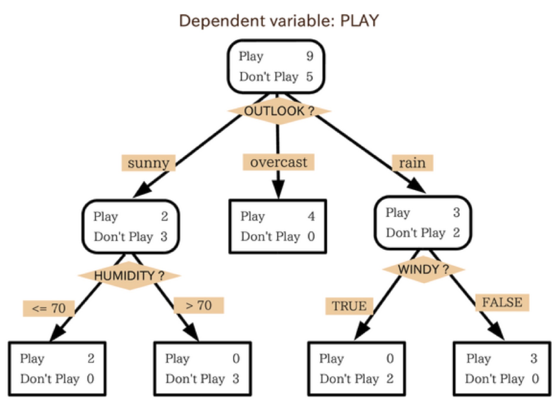
Then you train a whole 'forest' of these decision trees on random subsets of your data so they don't all learn the same features and they don't overfit

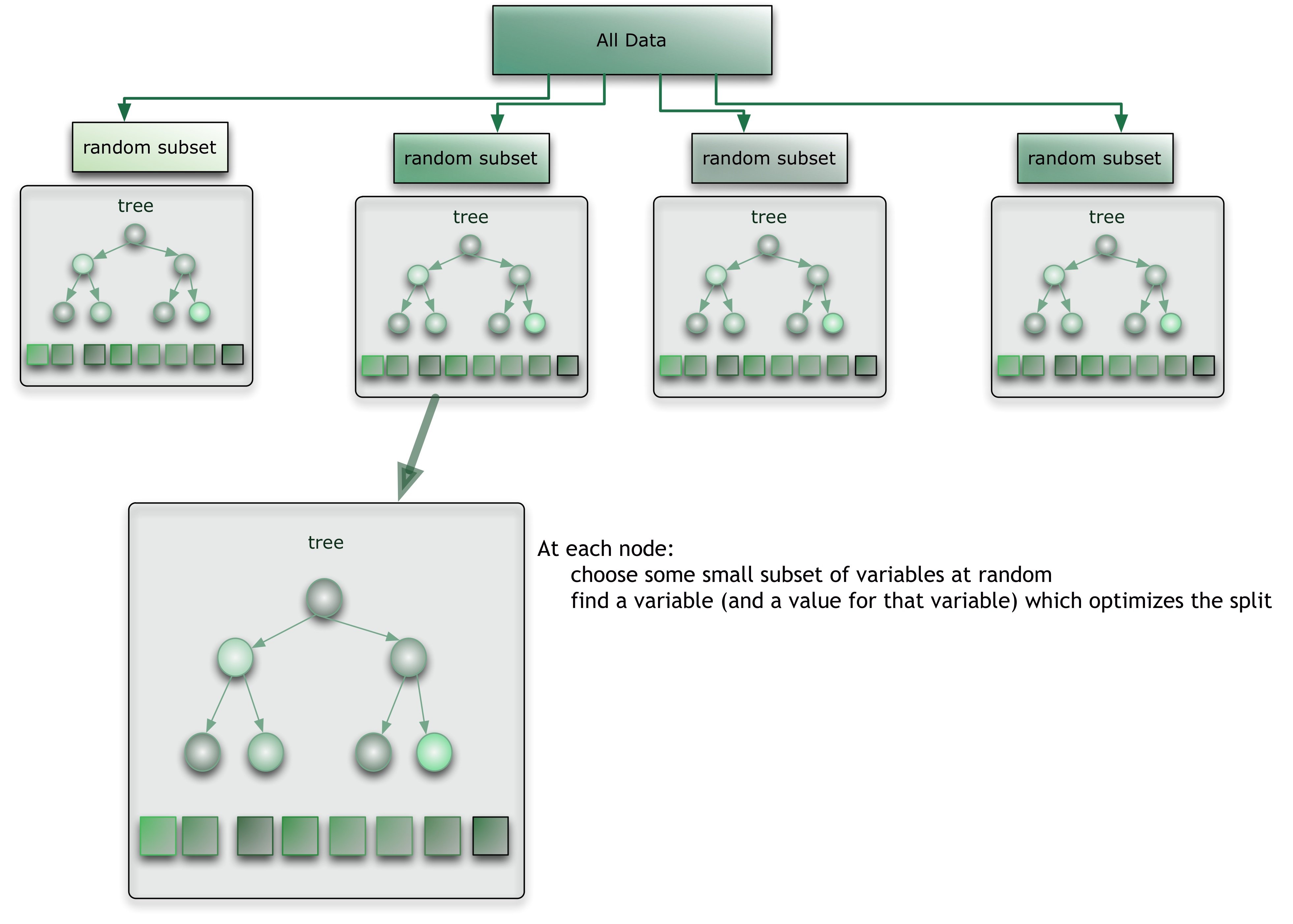
Source: Citizennet.com

Random Forests in Action

Most machine learning algorithms implemented in scikit-learn expect a numpy array as input X. The expected shape of X is (n_samples, n_features)

Supervised Learning also needs as input an array Y, the labels of the data

We'll also split the data in a training and testing set.

Never ever ever ever learn on test data

The classifiers learn the patterns in your data and if you test how well the classifier works on the data you used to train it, off course its going to work well. But then you present it with new data and suddenly your performance can go down the drain. Even better would be to make split your training data even further (check out cross-validation) and take the model that performs best on all the different splits of your data. Seriously, go read the docs on this.

Source: Scikit-Learn Tutorial

Here are Dropbox links to the two files and the notebook this was created in:

• IPython Notebook
• classify X_train.csv
• classify X_test.csv

    import pandas as pd

    # Let's load the data from some CSV files I prepared
    # The training data contains the data of (only) 4 dogs
    X_train = pd.read_csv("classify X_train.csv", index_col=0)
    # The testing data contains the data of the remaining 29 dogs
    X_test = pd.read_csv("classify X_test.csv", index_col=0)

    # My Y's are simply a column called "label" inside my X's

    n_samples, n_features = X_train.shape
    print("Training Samples: {:<4}, Features: {}".format(n_samples, n_features))

    n_samples, n_features = X_test.shape
    print("Testing  Samples: {:<4}, Features: {}".format(n_samples, n_features))

    Training Samples: 486 , Features: 32
    Testing  Samples: 3236, Features: 32

Normally you can take 50-50 splits or 80-20, especially if you want to do Cross Validation, but this seemed to work just fine.

As you can see, there are 32 features which basically describe the following:

• max_force = the peak of the force that paw applied to the ground. The ratio between front and hind paws seems to be about 60:40 so this should give it a way to estimate whether its a front or hind paw
• max_surface = the peak of the contact surface area of the paw. Again, the front paws are almost always a bit larger, probably because they also have to bear more force and are compressed more, so again a nice feature for separating front and hind paws.
• max_duration = the number of frames the paw was in contact with the ground. This isn't particularly useful, but it might put the difference in frames between paws in perspective

Then for each paw, we look backwards and forwards 2 paws and calculate the same features (f, s, m) but we also add the distance in x (width), y (length) and z (frames). This basically tells you where the other paw was located relative to the current one. Given that the pattern is highly repeatable, I have high hopes this will work well.

For the first two and last two paws, there may not be 1 or 2 paws in front or behind it, so I'll fill those numbers with NaN's for now.

cols = ['max_force', 'max_surface', 'max_duration',
        '-f2', '-s2', '-m2', '-x2', '-y2', '-z2',
        '-f1', '-s1', '-m1', '-x1', '-y1', '-z1',
        'f1',  's1',  'm1',  'x1',  'y1',  'z1',
        'f2',  's2',  'm2',  'x2',  'y2',  'z2']

The features

So for the yellow encircled paw, we calculate the x and y distances. The white line connecting the paws shows the chronological order.

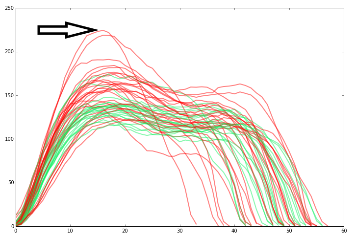
Here I added a plot of the total force (for the whole paw) for each frame. Red are the right front paws, green are the left front paws. For now, we'll just use the peak value.

from sklearn.ensemble import RandomForestClassifier

# So we create a class instance, without any hyperparameters, we'll get to that later
rf = RandomForestClassifier()
# We fit a model on the training data, using only the feature columns and we drop any columns that contain NaN's
# Because of I have to drop the NaN's I have to make sure I also drop them from my labels column, so it looks a bit clunky
rf.fit(X_train[cols].dropna(),
        X_train[cols+["label"]].dropna()["label"])

score = rf.score(X_test[cols].dropna(),
                    X_test[cols+["label"]].dropna()["label"])
print "Score: {:.2f}".format(score)

Score: 0.93

Ways to improve performance

We scored 93%! Which is most likely better than the interns that labeled the data for me! Apparently there are such strong patterns in the data that it already works really well on such a small data set.

Since the Random Forest is indeed random, the score I get above here seems to vary slightly each time I run it. There are probably flags to prevent this behavior, but its more fun this way :-)

Since my example data has a lot of samples (~800, so about 25%) that contain NaN, so we'll replace them with the mean using Imputation. You could get more fancy and use regression to predict what values I should replace them with, but we'll keep it simple. Actually, the way I'm imputing the values is wrong, because I'm replacing it with the mean along all the columns, even though there are huge differences based on the size of the dog. A better way would be to group the dataframe by dog and then impute the values, but again: let's keep it simple.

We also ran the Random Forest without hyperparameters, so we'll use better settings. I got these using a Grid Search that checked 216 different combinations of hyperparameters on a slightly bigger portion of the data. Grid Search can also perform Cross-Validation, so I'm relatively confident that these hyperparameters will give a better result

%matplotlib inline
from sklearn.preprocessing import Imputer
from sklearn.metrics import confusion_matrix

# We use the Imputer class to replace NaN's with the mean, calculated along the columns
imputer = Imputer(missing_values="NaN",
                    strategy="mean", axis=0)

X_train2 = X_train.copy()
X_train2[cols] = imputer.fit_transform(X_train[cols])
X_test2 = X_test.copy()
X_test2[cols] = imputer.fit_transform(X_test[cols])

# Notice that there are now a bunch of hyperparameters in here
rf = RandomForestClassifier(bootstrap=False, min_samples_leaf=3,
                            min_samples_split=3, criterion='gini',
                            max_features=10, max_depth=None)

# We fit and score again and get a new (high) score
rf.fit(X_train2[cols], X_train2["label"])
score = rf.score(X_test2[cols], X_test2["label"])
print("New score: {:.2f}".format(score))

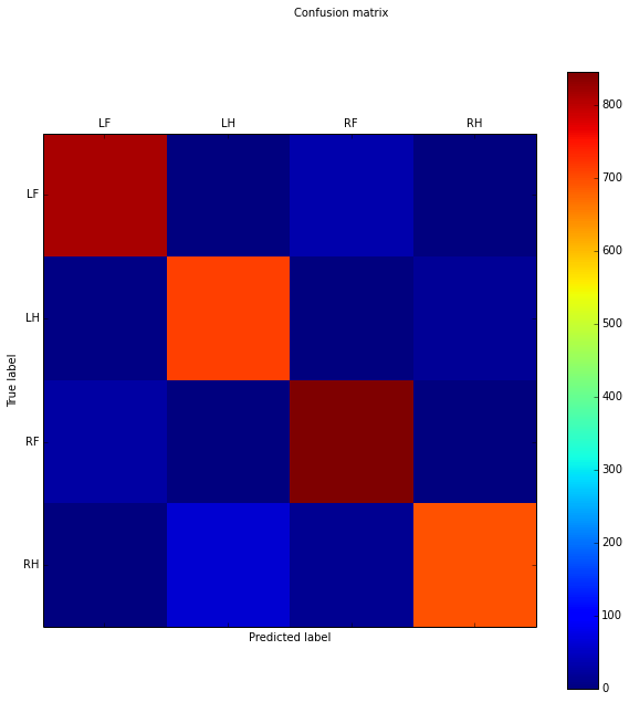
# Compute confusion matrix
y_pred = rf.predict(X_test2[cols])
cm = confusion_matrix(X_test2["label"], y_pred)
print(cm)

import matplotlib.pyplot as plt
fig, ax = plt.subplots(figsize=(10,10))
cax = ax.matshow(cm)
fig.suptitle("Confusion matrix")
fig.colorbar(cax)
ax.set_ylabel('True label')
ax.set_xlabel('Predicted label')
ax.set_xticks(range(4))
ax.set_xticklabels(["LF","LH","RF","RH"])
ax.set_yticks(range(4))
_ = ax.set_yticklabels(["LF","LH","RF","RH"])

New score: 0.95
    [[812   1  36   0]
    [  5 710   3  17]
    [ 28   3 845   0]
    [  3  61  16 696]]

Evaluating the results

This time we score slightly higher: 95%, but on the whole 100% of the dataset. It seems it systematically get's certainly samples wrong, so tuning the parameters and imputating values won't really help here.

By looking at the confusion matrix, we see on the diagonal that it did a kick ass job of predicting most right. Then interestingly enough, there are some superdiagonal which also have 30-60 errors. It turns out, sometimes when you give it a Right Front (RF) sample, it gets labeled as a Left Front (LF) sample or vice versa. The same thing happens for the hind paws. So clearly, it would help to have better features that distinguish between left and right.

I'm also curious how well it performs on each separate dog in our testing set, perhaps there are some outliers.

import numpy as np

subject_scores = []
min_score = 1.0
min_measurement = ""
min_subject = ""
group = None
print("Subject id\tWeight\tSamples\tMean +/- STD")
for subject_id, subject_group in X_test2.groupby("subject_id"):
    scores = []
    weight = subject_group["weight"].unique()[0]
    samples = len(subject_group)
    for measurement_id, measurement_group in subject_group.groupby("measurement_id"):
        score = rf.score(measurement_group[cols], measurement_group["label"])
        scores.append(score)
        if score < min_score:
            min_score = score
            min_measurement = measurement_id
            min_subject = subject_id
            group = measurement_group
    arrow = ""
    if np.mean(scores) < 0.9:
        arrow = "<-"
    print("{:<10}\t{:<2}\t{:<3}\t{:.2f} +/- {:.2f} {}".format(subject_id, weight, samples, np.mean(scores), np.std(scores), arrow))
    subject_scores.append(np.mean(scores))

print("Worst score: {:.2f} for {} in {}".format(min_score, min_subject, measurement_id[:5]))

Subject id Weight Samples Mean +/- STD
subject_0  30 86  0.96 +/- 0.07
subject_10 9  178 1.00 +/- 0.00
subject_12 50 83  0.91 +/- 0.14
subject_13 51 74  1.00 +/- 0.00
subject_14 21 101 0.97 +/- 0.11
subject_15 5  193 0.95 +/- 0.04
subject_16 16 123 1.00 +/- 0.00
subject_17 31 84  0.99 +/- 0.05
subject_18 9  199 0.98 +/- 0.03
subject_19 26 111 0.95 +/- 0.09
subject_2  59 61  1.00 +/- 0.00
subject_20 64 57  1.00 +/- 0.00
subject_21 22 82  0.98 +/- 0.05
subject_22 17 103 0.98 +/- 0.04
subject_23 25 89  0.96 +/- 0.10
subject_24 4  229 0.94 +/- 0.04
subject_25 41 97  0.98 +/- 0.04
subject_26 4  178 0.79 +/- 0.13 <-
subject_27 6  154 0.84 +/- 0.13 <-
subject_28 2  141 0.80 +/- 0.11 <-
subject_29 69 59  0.87 +/- 0.24 <-
subject_35 5  189 0.97 +/- 0.04
subject_36 43 80  0.95 +/- 0.08
subject_4  7  158 0.98 +/- 0.03
subject_5  57 64  0.92 +/- 0.17
subject_6  54 50  1.00 +/- 0.00
subject_7  37 69  1.00 +/- 0.00
subject_8  62 52  0.98 +/- 0.07
subject_9  34 92  1.00 +/- 0.00
Worst score: 0.29 for subject_29 in svr_3

For each dog, I printed out their weight and their mean/std score. This was calculated on each measurement, perhaps there are just some measurements where it performs poorly.

If the score dropped below 90% I added a small <- behind it and as we can see there are at least 4 dogs where it performs more poorly. However, in three of these dogs it has to classify between 141-178 samples, so getting at least 80% right of those is still pretty impressive. On our biggest (or at least heaviest) dog it got 87% right, but out of only 59 measurements. This dog is probably too big for the plate, so you get much less samples out of each measurements. Also, a lot of his steps are on the edge of the plate, which I didn't try to predict in this analysis.

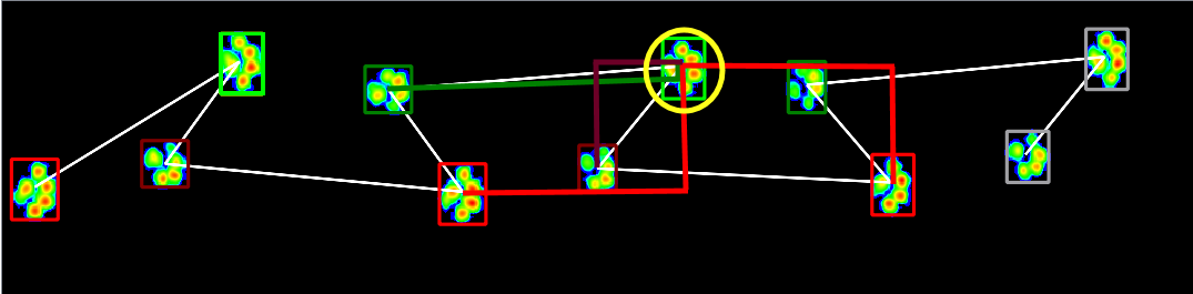
I also looked up the worst measurement, but again randomness made sure that it didn't align with the example I cooked up below. Because it has some incomplete steps, it was a bit of a hassle to show that one, so instead we'll show one of his other measurements instead:

import tables
import sys
sys.path.append("C:\Dropbox\Development\AnalyzingDogs")
import data_mangling

table = tables.open_file("C:\Dropbox\Development\Experiments\data.h5", "a")
contacts, contact_dict, measurements = data_mangling.get_contacts(table, subject_id="subject_29")

measurement_id = "ser_2 - 19-4-2010 - Entire Plate Roll Off"
measurement = measurements[measurement_id]
contacts = contact_dict[measurement_id]
group = X_test2[(X_test2["subject_id"]=="subject_29").values & (X_test2["measurement_id"]==measurement_id).values]
prediction = rf.predict(group[cols])


fig, ax = plt.subplots(figsize=(16, 6))
valid_index = 0
x = []
y = []
for index, contact in enumerate(contacts):
    minx = contact["min_x"]
    maxx = contact["max_x"]
    miny = contact["min_y"]
    maxy = contact["max_y"]
    x.append(np.mean([minx, maxx]))
    y.append(np.mean([miny, maxy]))
    ax.plot([minx, minx, maxx, maxx, minx],
            [miny, maxy, maxy, miny, miny],
            color=["#11F05F","#008000", "#FF0000","#800000"][prediction[index]],
            linewidth=5)
    ax.plot([minx-1, minx-1, maxx+1, maxx+1, minx-1],
            [miny-1, maxy+1, maxy+1, miny-1, miny-1],
            color=["#11F05F","#008000", "#FF0000","#800000"][contact["contact_label"]],
            linewidth=5)

ax.plot(x, y, linewidth=3, color="w")
ax.imshow(measurement["data"].max(axis=2).T);
ax.set_xticks([])
_ = ax.set_yticks([])

The white line again connects the paws in chronological order. The color on the inside it was the algorithm predicted, the color on the outside is what it should have been. It basically just tries LH, RF everywhere, so by chance it got that right at least once.

The problem seems to be that the dog walked diagonally, which causes left and right to cross over. His previous and next right front paw don't even hit the plate, because his strides are that long, so its not hard to imagine why the classifier got it wrong. Obviously, adversarial samples like this can give hints to what features I should incorporate to make it more robust.

Visualize the Random Forest

Finally, we can export the tree and visualize its structure

import StringIO
import pydot
from sklearn import tree
from IPython.core.display import Image

# Visualize one of the trees
dot_data = StringIO.StringIO()
tree.export_graphviz(rf.estimators_[0], out_file=dot_data)
graph = pydot.graph_from_dot_data(dot_data.getvalue())
image = graph.write_png("./images/random_network.png")

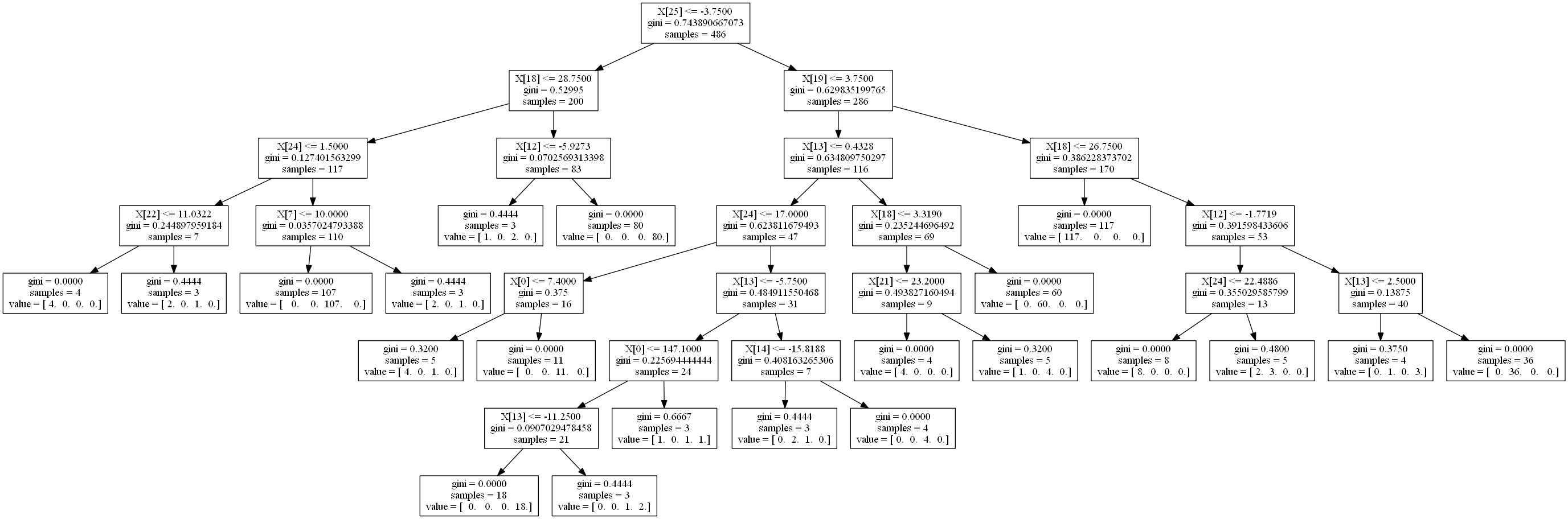
The questions it asks are basically:

• Is the second next paw less than -3.75 in front of me?
• Left: Then is the next paw less than 28.75 to the right of me?
  • Left: Is that second next paw less than 1.5 to the right of me? (You're probably a Right Front)
  • Right: Or is the previous paw less than 10 to the right of me? (You're probably a Right Hind)
• Right: Or is the next paw less than 3.75 ahead of me?
  • Left: Is the previous paw less than 0.43 in front of me? (This branch is the deepest, mostly right paws)
  • Right: Is the next paw less than 26.75 to the right of me?
  • Left: You're a Left Front
  • Right: If the previous paw is less than 2.5 ahead of me, you're Left Hind

If I had to write some kind of state machine to decypher it, I'm not sure if this would be what I would come up with

# Here's the index (used in the image of the tree), with the feature name and importance
for i,j,k in sorted(zip(range(len(cols)), cols, rf.feature_importances_), key=lambda x: x[2], reverse=True):
    print "{:<2} {:<12} {:.4f}".format(i,j,k)

12 -x1          0.2180
19 y1           0.2179
25 y2           0.1708
18 x1           0.1153
13 -y1          0.1084
7  -y2          0.1035
24 x2           0.0188
6  -x2          0.0151
10 -s1          0.0061
1  max_surface  0.0051
11 -m1          0.0027
20 z1           0.0024
22 s2           0.0024
14 -z1          0.0022
16 s1           0.0020
2  max_duration 0.0017
5  -m2          0.0017
3  -f2          0.0015
15 f1           0.0010
26 z2           0.0008
0  max_force    0.0008
23 m2           0.0007
8  -z2          0.0005
9  -f1          0.0004
21 f2           0.0002
17 m1           0.0000
4  -s2          0.0000

Take home message

Machine Learning isn't going to bite you. While there are plenty of mistakes you can make and things that can go wrong, as I've hopefully shown you can get a really good performing classifier with relative ease.

Check out the Scikit-Learn docs and just try it at home!

Questions?